Query Workbench
The Query Workbench provides a rich graphical user interface to perform query development.
Using the Query Workbench, you can conveniently explore data, create, edit, run, and save N1QL queries, view and save query results, and explore the document structures in a bucket - all in a single window.
Features of the Query Workbench include:
-
A single, integrated visual interface to perform query development and testing.
-
Easy viewing and editing of complex queries by providing features such as multi-line formatting, copy-and-paste, syntax coloring, auto completion of N1QL keywords and bucket and field names, and easy cursor movement.
-
View the structure of the documents in a bucket by using the N1QL INFER command. You no longer have to select the documents at random and guess the structure of the document.
-
Display query results in multiple formats: JSON, table, and tree. You can also save the query results to a file on disk.
| The Query Workbench is only available on clusters that are running the Query Service. |
Accessing the Query Workbench
If a cluster is running the Query Service, the Query Workbench can be found under the cluster’s Advanced > Query Workbench tab.
-
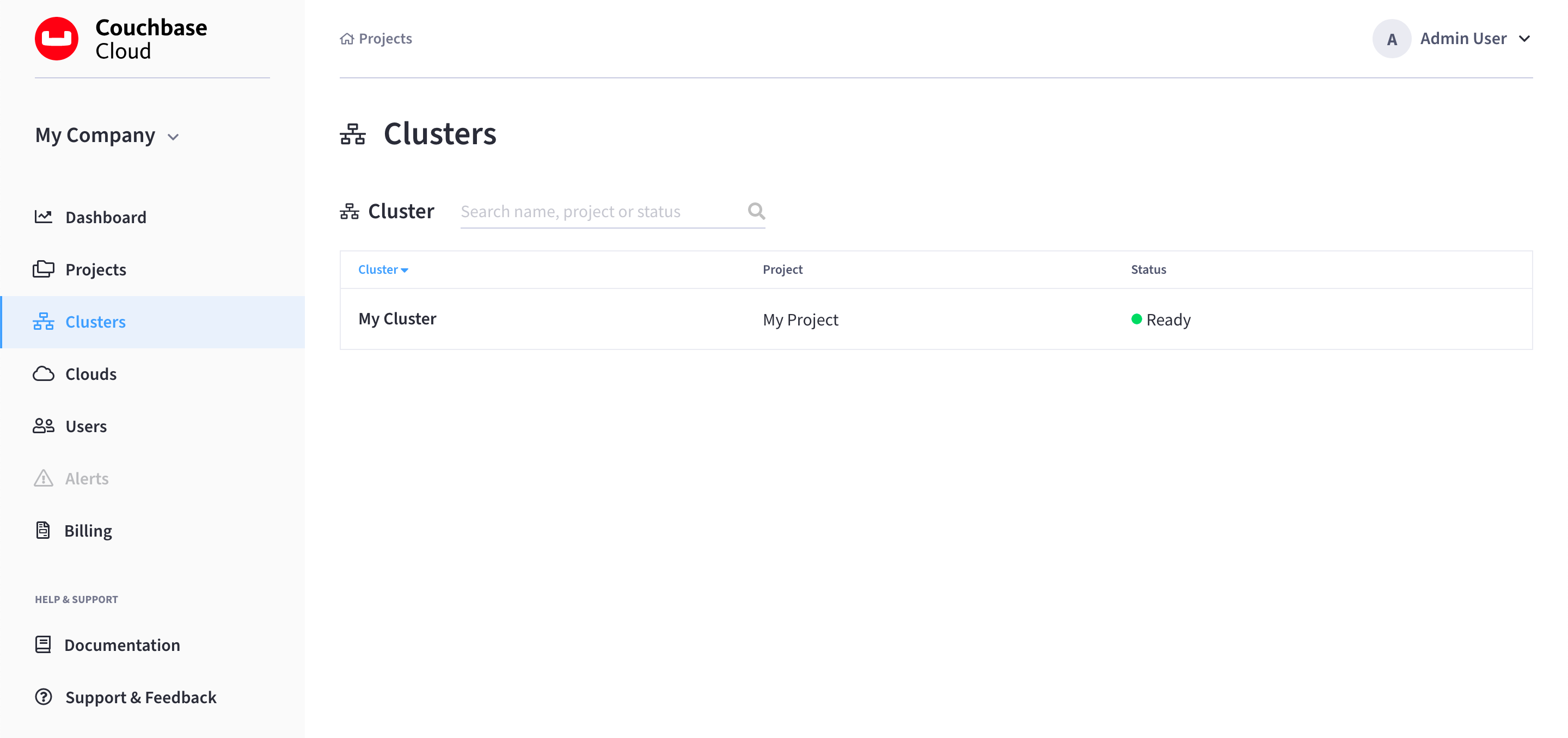
Go to the Clusters tab.
-
Find and click on your cluster.
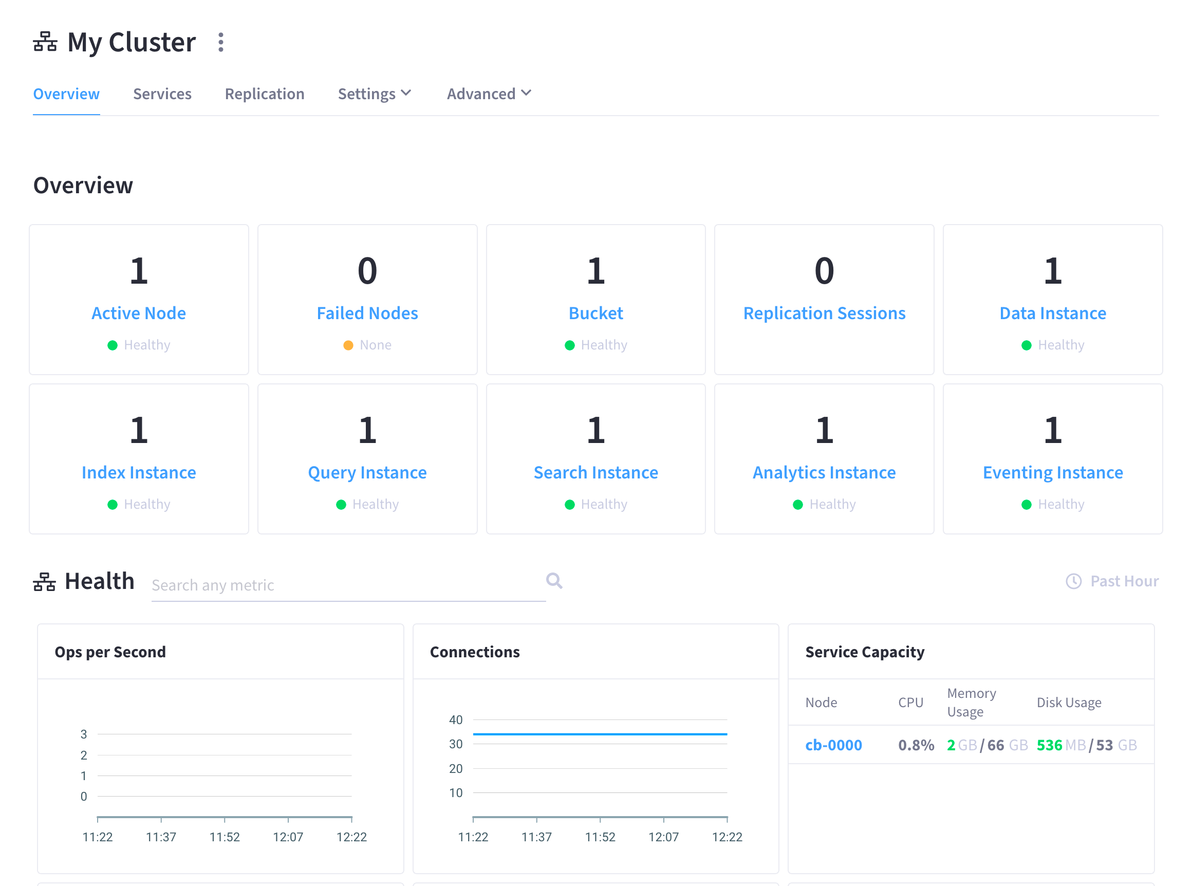
This opens the cluster’s Overview tab:
-
Go to the Advanced > Query Workbench tab.
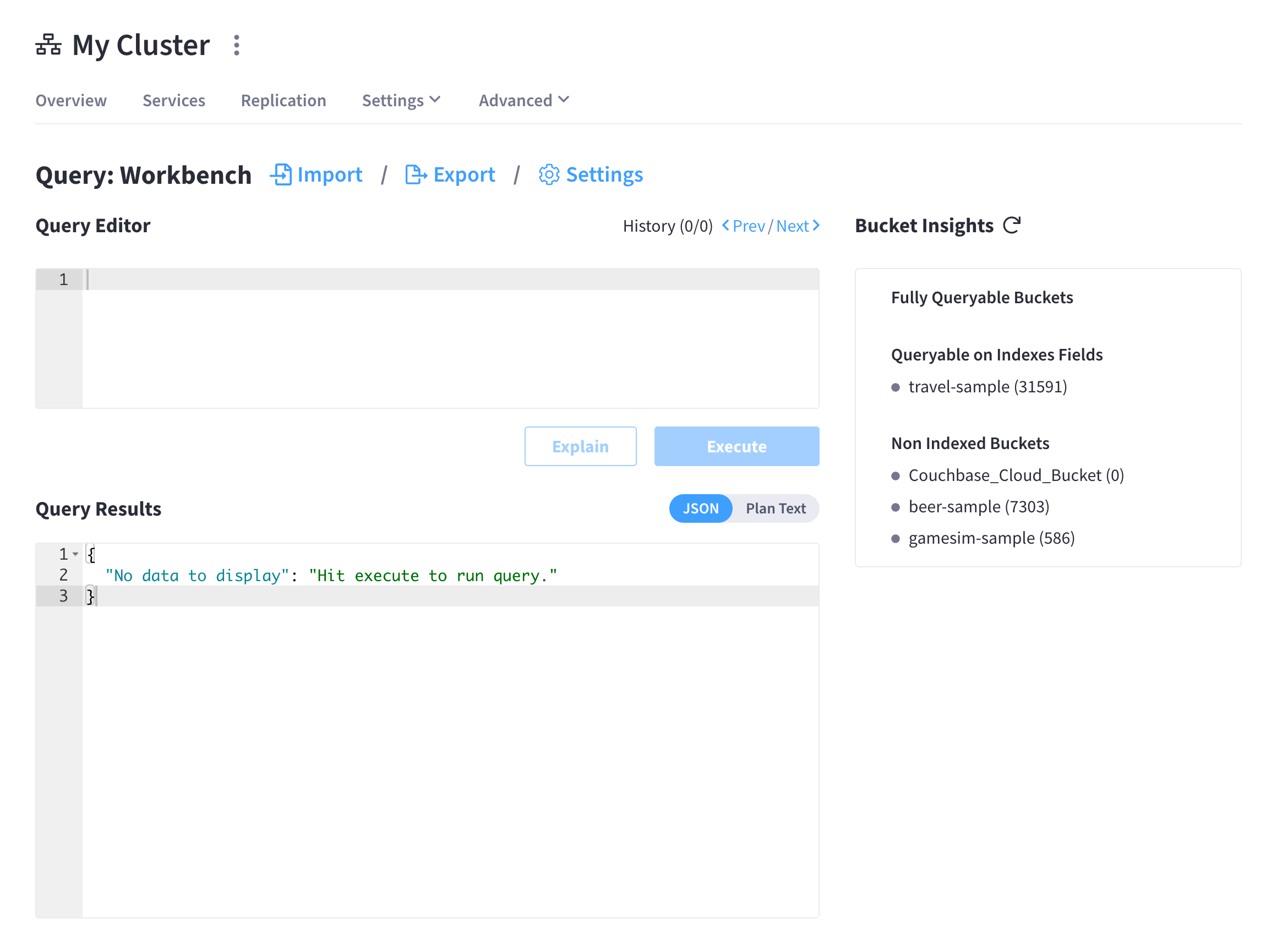
The Query Workbench consists of three working areas as shown in the following figure:
Using the Query Editor
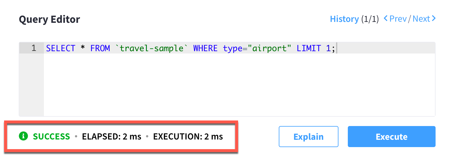
The Query Editor is where you build and run queries, and view query execution plans. Enter a query into the Query Editor, and then run the query by clicking Execute.
You can also execute queries by typing a semi-colon (;) at the end of the query and hitting Enter.
|
The Query Editor provides the following additional features:
-
Syntax coloring - For easy viewing, N1QL keywords, numbers and string literals are differently colored.
-
Auto-completion - When entering a keyword in the Query Editor, if you press the Tab key or Ctrl+Space, the tool offers a list of matching N1QL keywords and bucket names that are close to what you have typed so far. For names that have a space or a hyphen (-), the auto-complete option includes back quotes around the name. If you expand a bucket in the Data Bucket Analysis, the tool learns and includes the field names from the schema of the expanded bucket.
-
Support for N1QL INFER statements - The tool supports the N1QL INFER statement.
Run a Query
After entering a query, you can execute the query either by typing a semicolon (;) and pressing Enter, or by clicking the Execute button.
When the query is running, the Execute button changes to Cancel, which allows you to cancel the running query.
When you cancel a running query, it stops the activity on the cluster side as well.
| The Cancel button does not cancel index creation statements. The index creation continues on the server side even though it appears to have been canceled from the Query Workbench. |
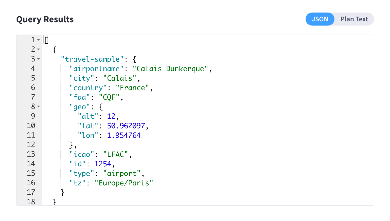
Viewing the Query Results
When you execute a query, the results are displayed in the Query Results area. Since large result sets can take a long time to display, it’s recommended that you use the LIMIT clause as part of your query when appropriate.
The figures in this section display the result of the following query:
SELECT * FROM `travel-sample` WHERE type="airport" LIMIT 1;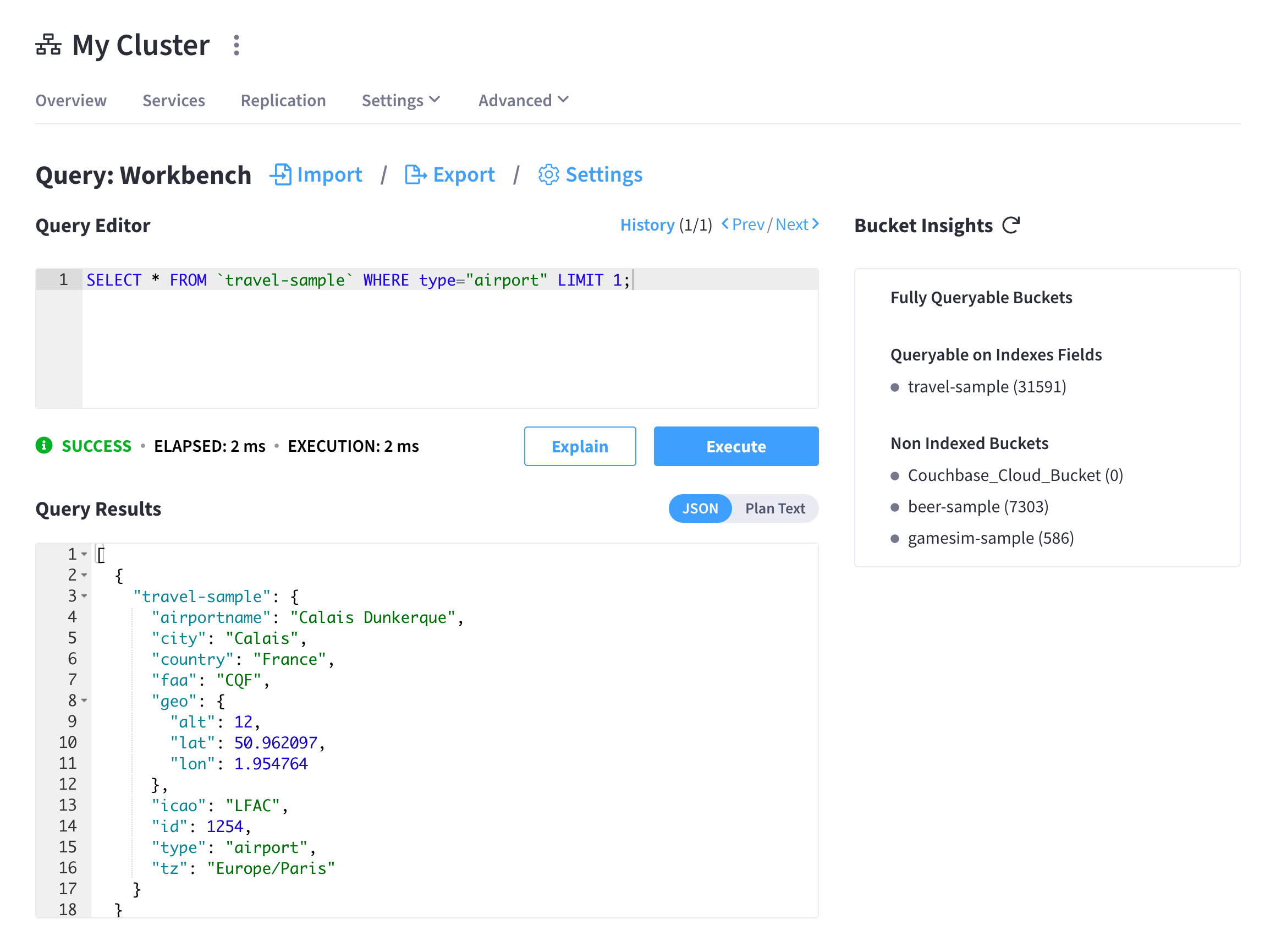
When a query finishes, the query metrics for that query are displayed between the Query Editor and the Query Results areas.
-
Status - Shows the status of the query. The values can be: success, failed, or HTTP codes.
-
Elapsed - Shows the overall query time.
-
Execution - Shows the query execution time.
-
Result Count - Shows the number of returned documents.
-
Mutation Count - Shows the number of documents deleted or changed by the query. This appears only for UPDATE and DELETE queries instead of Result Count.
-
Result Size - Shows the size in bytes of the query result.
JSON Format
JSON, where the results are formatted to make the data easy to read. You can also expand and collapse objects and array values using the small arrow icons next to the line numbers.
If you clicked Execute, the results of the query are shown. If you clicked Explain, the results are the same as Plan Text format.
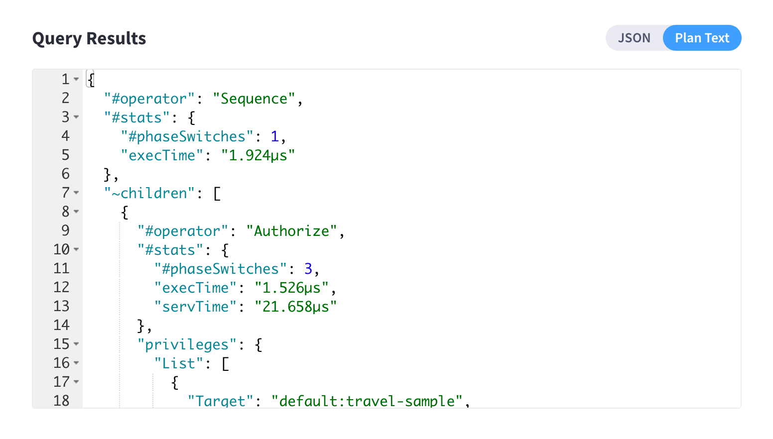
Plan Text
The Plan Text tab shows the EXPLAIN query execution plan in JSON format.
If you clicked Execute, a detailed query execution plan is shown, which includes information about how long each step in the plan took to execute. If you clicked Explain, the intended query execution plan is shown (minus the details that would be included if you actually executed the query).
View Query History
The Query Workbench maintains a history of all the queries executed. The currently shown position in the history is indicated by the numbers next to the history link. For example, (151/152) indicates that query #151 is currently shown, out of a total history length of 152 queries. Use the <Prev / Next> links at the top of the editor to navigate through the history.
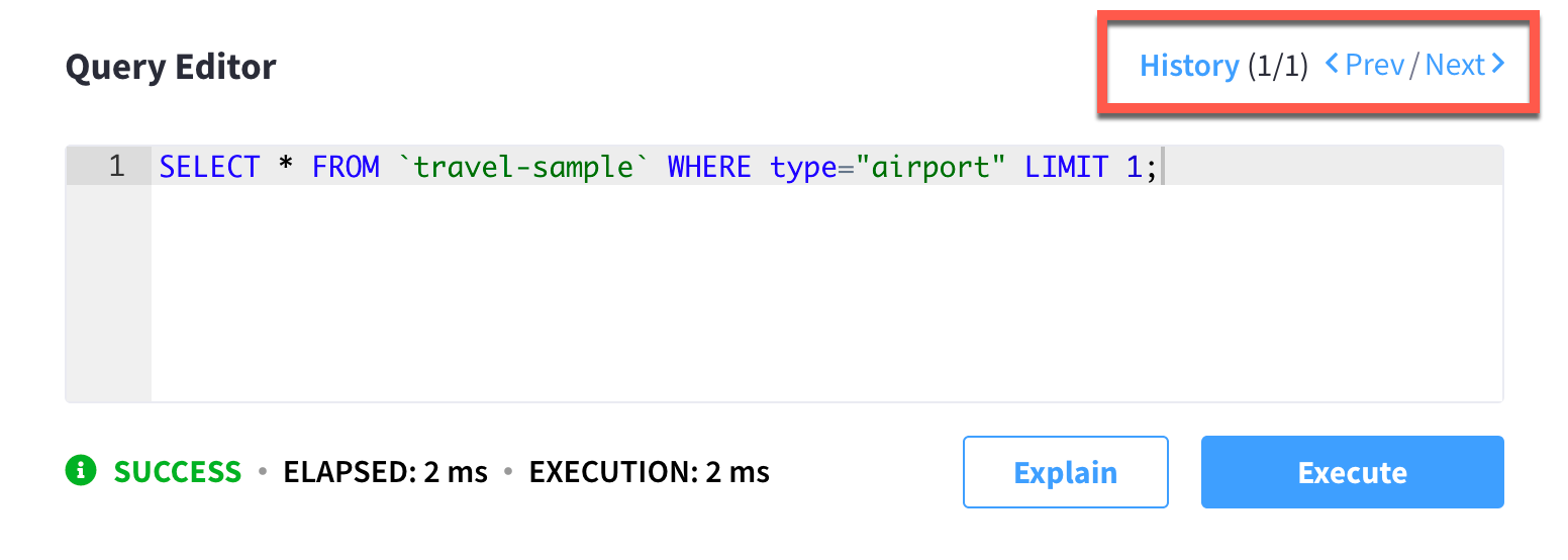
If you edit a previous query and execute it, the new query is stored at the end of the history. The history is persistent across browser sessions. The query history only saves queries; due to limited browser storage it does not save query results. Thus, when you restart the browser or reload the page, you can see your old queries, but you must re-execute the queries if you want to see their results.
| Clearing the browser history clears the history maintained by the Query Editor as well. |
Clicking the History link (next to the <Prev / Next> links) opens the Query History fly-out menu:
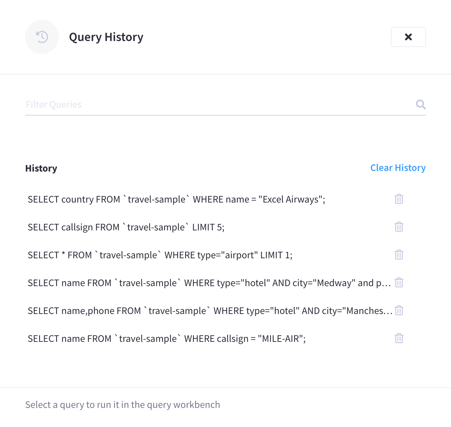
You can scroll through the entire query history, and click on an individual query to be taken to that particular point in the history.
-
Search history - You can search the query history by entering text in the Filter Queries search box. All matching queries are displayed.
-
Delete a specific entry - Click the Trash icon next to a particular query to delete it from the history.
This can be useful if you want a more manicured history for when you’re exporting it for future use. -
Delete all entries - Click Clear History to delete the entire query history.
Import Query
You can load a query from a file into the Query Editor. Click Import to open the Import Query History fly-out menu.
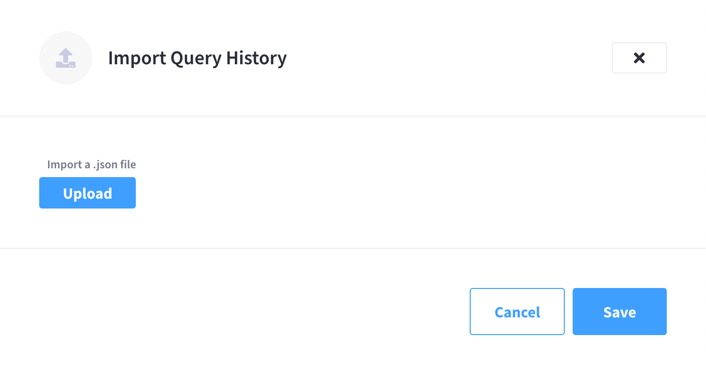
Click Upload and then select a local .json file that you wish to import.
After clicking Save, the content of the file is added to the Query Editor history.
Export Query History and Results
You can export the query history and/or results in a variety of formats. Click Export to open the Export fly-out menu.
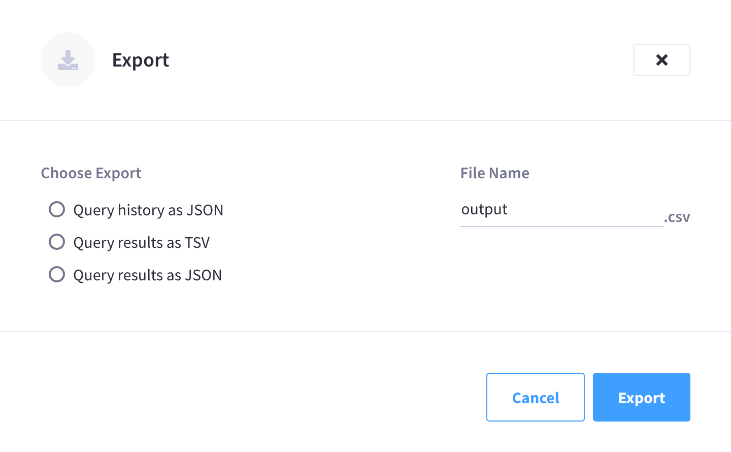
Use the radio buttons to choose whether to export query history or query results in one of the available formats. Enter a name for the exported file and click Export.
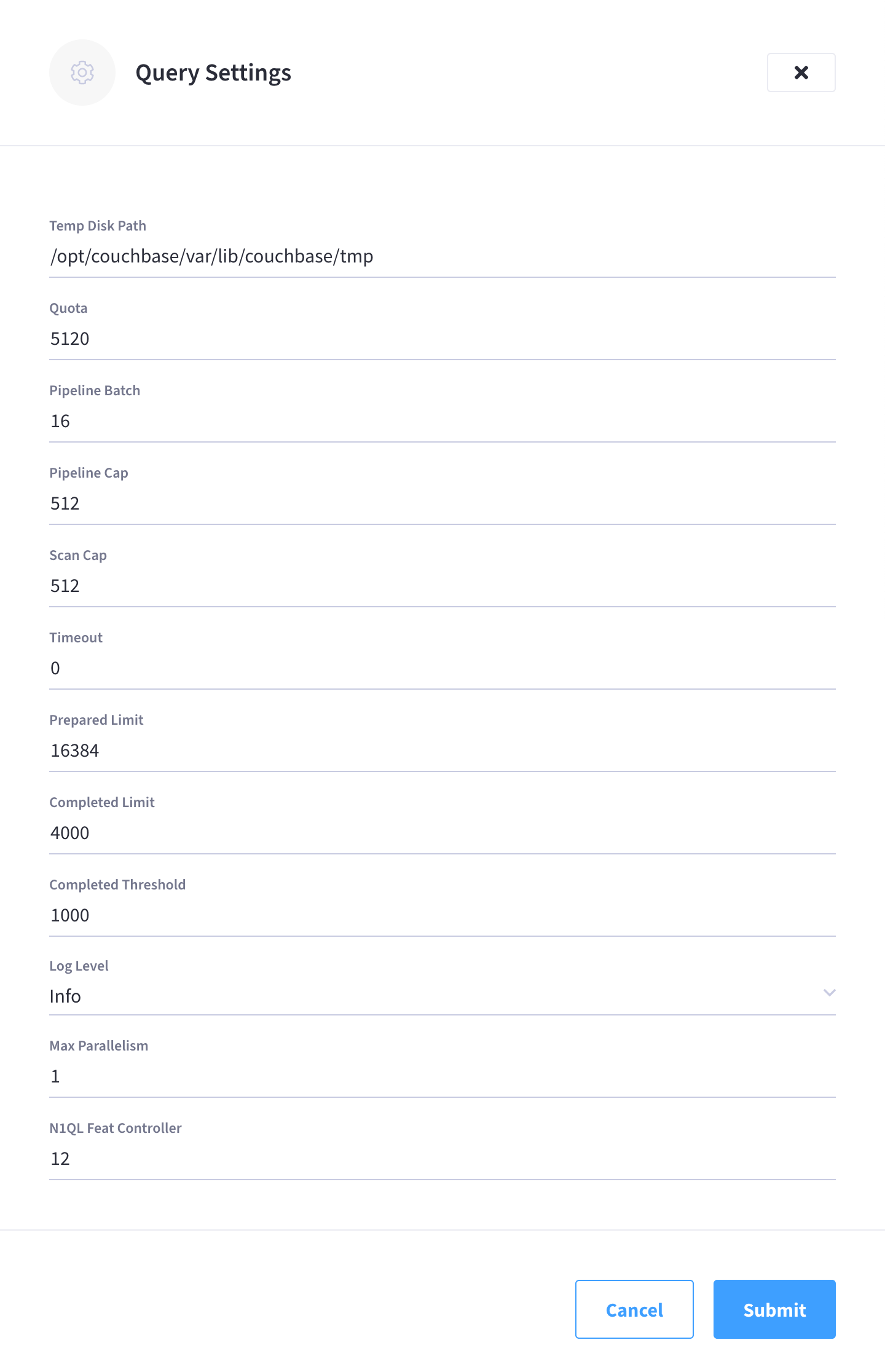
Query Settings
Clicking Settings opens the Query Settings fly-out menu, which contains several settings for configuring the Query Service.
-
Query Temp Disk Path: Allows specification of the path to which temporary files are written, based on query activities.
-
Quota: The maximum size for the Query Temp Disk Path, in megabytes.
-
Pipeline Batch: The number of items that can be batched for fetches from the Data Service.
-
Pipeline Cap: The maximum number of items that can be buffered in a fetch.
-
Scan Cap: The maximum buffered channel size between the indexer client and the Query Service, for index scans.
-
Timeout: The maximum time to spend on a request before timing out.
-
Prepared Limit: The maximum number of prepared statements to be held in the cache.
-
Completed Limit: The number of requests to be logged in the completed requests catalog.
-
Completed Threshold: The completed-query duration (in millisconds) beyond which the query is logged in the completed requests catalog.
-
Log Level: The log level used in the logger.
-
Max Parallelism: The maximum number of index partitions for parallel aggregation-computing.
-
N1QL Feature Controller: Provided for technical support only.
Click Submit to save any configuration changes to the above settings.
For more information about these settings, refer to the N1QL Admin REST API.
Data Insights
The Bucket Insights area displays all installed buckets in the cluster. By default, when the Query Workbench is first loaded, it retrieves a list of available buckets from the cluster. The Bucket Insights area is automatically refreshed when buckets or indexes are added or removed, but you can manually refresh it using the refresh button.
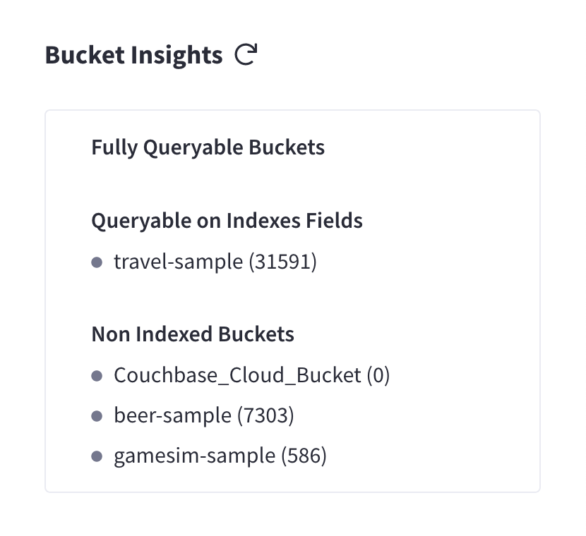
The buckets are grouped into the following categories based on the indexes created for the bucket:
-
Fully Queryable Buckets: Contain a primary index or a primary index and secondary indexes.
-
Queryable on Indexed Fields: Do not contain a primary index, but have one or more secondary indexes.
-
Non-Indexed Buckets: Do not contain any indexes. These buckets do not support queries. You must first define an index before querying these buckets.
You can expand any bucket to view the schema for that bucket: field names, types, and if you hover the mouse pointer over a field name, you can see example values for that field. Bucket analysis is based on the N1QL INFER statement, which you can run manually to get more detailed results. This command infers a schema for a bucket by examining a random sample of documents. Because the command is based on a random sample, the results may vary slightly from run to run. The default sample size is 1000 documents. The syntax of the command is:
INFER bucket-name [ WITH options ];where options is a JSON object, specifying values for one or more of sample_size, similarity_metric, num_sample_values, or dictionary_threshold.
For example, to increase the sample size to 3000, you could use the following query:
INFER `travel-sample` WITH {"sample_size":3000};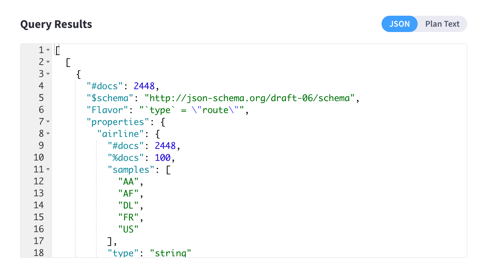
INFER `travel-sample` WITH {"sample_size":3000};